The compensated demand curve indicates the quantity of a good that a consumer would buy if he is income-compensated for a change in the price of that good. In other words, the compensated demand curve for a good shows the amount of quantity purchased by the consumer if the income effect is removed.
The compensated demand curve can explain both the Hicks and Slutsky approaches to the substitution effect. The two-story Figure 45 (A) illustrates the construction of the Hicks and Slutsky compensated demand curves and the uncompensated (or ordinary or Marshallian) demand curve.
The upper portion of the figure depicts the substitution effect of the Hicks and Slutsky analyses and the combined price effect.
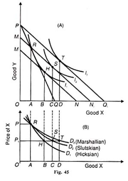
The lower portion of the figure shows the derivation of the Hicks and Slutsky compensated demand curves and the standard demand curve. First, consider the lower diagram (B), where the price of good X is taken on the vertical axis. Point P is an arbitrary point on this axis that shows X’s price when the budget line is PQ in the upper diagram. As shown by the budget line PQ1, the fall in the price of X is reflected in the lower diagram point P1.
The Marshallian Curve of Uncompensated Demand:
This section describes the derivation of the Marshallian uncompensated demand. The initial equilibrium of the consumer is at point R where the budget line PQ is tangent to the indifference curve I1 and OA of good X is bought by the consumer in the tipper diagram.
Let the price of X fall. As a result, the budget line PQ extends to PQ3, and the consumer is at a higher point of equilibrium T on the indifference curve I3. The movement from R to T is the price effect, including the substitution effect and the income effect, as shown by the D3 curve in the lower portion of the figure. This is the uncompensated (or ordinary or Marshallian) demand curve which shows that when the price of good X falls from P to P1, its quantity demanded increases from OA to OD.
The Hicksian Compensated Demand Curve:
Since the compensated demand curve is based on the substitution effect of a change in the price of good X, we carry the above analysis and derive the Hicks substitution effect. Let us take away the increase in the consumer’s real income due to the fall in the price of X equal to PM of good Y and Q1 N of X good by drawing a compensated budget line MN parallel to the budget line PQ1.
At point H, this line MN is tangent to the original indifference curve I1. The movement from point R to H on the I1 curve is the substitution effect that traces out the demand curve D1 in the lower portion of the figure when the demand for X increases from OA to OB with the fall in its price from P to P P1.
The Slutsky Compensated Demand Curve:
In order to derive the Slutsky substitution effect, let us take away the increase in the apparent real income of the consumer equal to PMX of Y and Q1N1 of X by drawing the Slutsky compensated budget line M1N1, parallel to PQ, which passes through the original point R on the I1, curve where he will buy the same quantity OA of X. But since the price of X has fallen, he will buy more of it so that he moves to point S on the higher indifference curve I2, which is tangent to the budget line
M1N1 Thus, the movement from R to S traces out the Slutsky compensated demand curve D2 in the lower part of the figure.
This curve shows that with the fall in the price of good X from P to P1, its demand increases from OA to ОС.
Conclusion:
The compensated demand curve D1 of Hicks and D2 of Slutsky show that the curve D2 is more elastic than D1. This is because the total expenditure on the purchase of good X is more significant in the Slutsky approach than in the Hicks approach. The conventional demand curve D3 is more elastic than even the Slutsky demand curve D2.
Another critical point is that the compensated demand curve, whether of Hicks or Slutsky, always slopes downward because it is drawn such that the substitution effect only is in operation. The income effect is altogether eliminated through compensating variation in income. But the standard demand curve may or may not slope downward. In the case of the standard demand curve like D, both substitution and income effects operate and explain the curve’s declining slope.
If X is an inferior good, the standard demand curve will slope downward but will be more elastic than the compensated demand curves D1 and D2 because the substitution effect is stronger than the income effect in the case of the standard demand curve. But if X happens to be a Giffen good, the standard demand curve will slope from left to right upward, i.e., it will have a positive slope because the income effect is stronger than the substitution effect. On the other hand, the compensated demand curves will have a negative slope because they are not affected by the income effect.